BarrierFormer: Transformer-Guided Predictive Barrier Enforcement for Safe Robot Control

Arizona State University
Conference on Robot Learning (CoRL) 2026

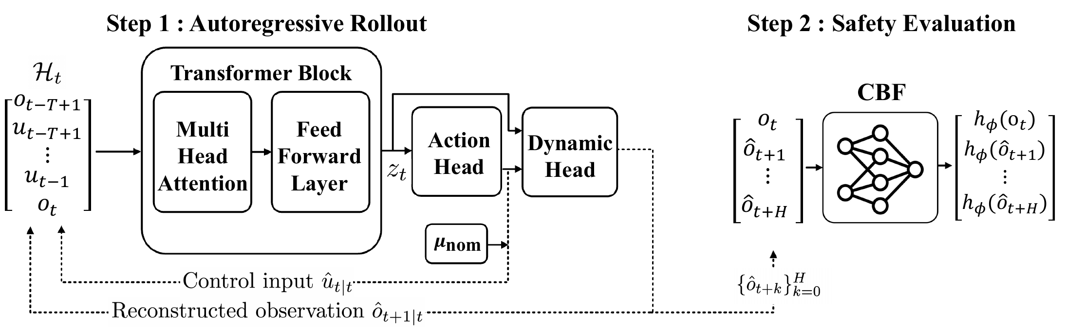
BarrierFormer operates in two steps during training. In Step 1, a causal transformer autoregressively generates a finite-horizon predictive rollout via the actor and dynamics heads. In Step 2, a barrier critic $h_\phi$ evaluates discrete-time CBF constraint violations along the predicted observations.

Abstract

Control barrier functions (CBFs) have become one of the most popular tools for encoding and enforcing state constraints in safety-critical robotics. Standard CBF approaches are inherently myopic in nature as they enforce safety only at the current time step. Consequently, the system can be driven toward the boundary of the safe set where no feasible safe control exists at a future timestep. Model predictive control (MPC) based approaches address this by enforcing state constraints over a receding horizon. However, such approaches generally require the model to be known for solving a constrained optimization problem at every step, which is computationally expensive for real-time deployment. We propose BarrierFormer, a barrier-supervised transformer framework that addresses these limitations by encoding rollout-level CBF constraints in learning a model-free safe policy. A causal transformer encodes observation-action history, autoregressively generates a predictive rollout through the dynamics head to replace the model, and provides a residual correction to a nominal controller through the action head to replace the online computation. A barrier critic operating on local observations evaluates CBF constraint violations along this rollout, and a safety teacher computes barrier-consistent actions satisfying these constraints as direct supervision targets for the learned control policy. During inference, the policy maps observation-action history to control actions without any online optimization or model knowledge, enabling real-time model-free predictive safety enforcement. Evaluations across linear and nonlinear, 2D and 3D dynamical systems for safe goal-directed navigation demonstrate that BarrierFormer outperforms existing reinforcement learning (RL)-based, diffusion-based, MPC-based, and transformer-based approaches in safety rate and inference latency.

Method

The agent has no prior knowledge of obstacle locations and perceives its environment through $n_\text{rays}$ evenly-spaced LiDAR rays within a fixed sensing radius $R$. A single observation is therefore insufficient to characterize the safety of the current state: the agent may be currently safe but on a trajectory toward an obstacle that has not yet entered its sensing range. BarrierFormer enforces the barrier condition over a predicted rollout rather than pointwise at the current state.
    • Problem setting: The agent follows $x_{t+1} = f(x_t) + g(x_t) u_t$ but observes only its own state, the goal-relative position, and radius-limited LiDAR returns. The policy sees just the observation-action history $\mathcal{H}_t$ of length $K$, and must reach the goal while keeping $d(p_t, R_j) \geq r$ for every obstacle.
    • Why pointwise CBFs fall short: The condition $h(F(x,u)) - h(x) + \alpha(h(x)) \geq 0$ constrains a single transition, so satisfying it at every step can still drive the system into a state where no safe action remains. BarrierFormer instead enforces $h_\phi(\hat{x}_{t+k+1}) \geq (1-\gamma)\, h_\phi(\hat{x}_{t+k})$ across a horizon $k = 0, \ldots, H-1$.
    • Step 1 — Autoregressive rollout: A GPT-2-style causal transformer encodes $\mathcal{H}_t$ into a latent $z_t$ feeding two heads: an actor head that outputs a residual correction to a nominal controller $\mu_\text{nom}$, and a dynamics head that predicts a state increment. Iterating the two generates the predictive rollout — standing in for the model that MPC would require.
    • Step 2 — Barrier critic: A critic $h_\phi$ maps each predicted observation to a barrier value, which is what makes it usable under partial observability. Per-step violations are aggregated across the horizon by a smooth log-sum-exp of the worst case.
    • SQP safety teacher: A sequential quadratic program computes the minimal correction to $\mu_\text{nom}$ that satisfies every horizon barrier constraint. Only its first action is kept, as the supervision target for the actor head. It runs during training only.
    • Data labeling: Because a collision-free state can still be doomed, a state is labeled safe only if it and the next $T_\text{label} = 32$ states are all collision-free; states in collision are labeled unsafe, and the rest stay unlabeled.
    • Training and deployment: All components train jointly under actor, dynamics, and barrier losses. At deployment, Step 2 is gone: the transformer maps history straight to actions — no SQP, no rollout, no online optimization, no model.
Seeing the Predicted Rollout

The predictive horizon, visualized. The left panel shows the full workspace: the agent (blue) executes the trajectory in solid blue toward the goal (green star), while the orange dashed line is the $H = 6$ step plan predicted by the transformer at that instant. The right panel zooms in on the agent, showing its LiDAR rays and the numbered steps of that predicted plan. This rollout is what the barrier critic evaluates during training — and it is precisely what a myopic, single-step CBF never looks at.

Double Integrator, $4 \times 4$ workspace, 12 obstacles.

BarrierFormer on the training distribution ($l = 4$ workspace, 8 obstacles). The agent perceives obstacles only through LiDAR rays within its sensing radius $R = 0.5$ and has no prior knowledge of obstacle locations. Safety is enforced purely by the policy parameters — no safety filter, no online optimization, and no model at inference.

Double Integrator (2D, linear)

Dubins Car (2D, nonlinear)

Evaluations

We evaluate BarrierFormer on three dynamical systems: one linear (Double Integrator, DI) and two nonlinear (Dubins Car, DC and Crazyflie, CF). The safety rate is the fraction of episodes in which the robot never collides with an obstacle; the reaching rate is the fraction in which it reaches its goal; the success rate requires both. All results are reported as mean $\pm$ std over 3 random seeds $\times$ 32 environments. We compare against four baselines spanning three model-free paradigms and one model-based paradigm: CBF-RL (RL-based), CoBL-Diffusion (diffusion-based), ConBaT (transformer-based), and MPC (model-based). All baselines are re-implemented in our framework using the same dynamics, observation model, and obstacle configurations.

Performance comparison in terms of safety rate (Safe), goal reaching rate (Reach), and per-step computational time (Time). Ours (Dyn-Head) generates predictive rollouts with the learned dynamics head, while Ours (Sim) uses the true simulator during training. Among model-free methods, Ours (Dyn-Head) achieves the best balance between safety and goal-reaching with competitive inference time. Among model-based methods, Ours (Sim) matches MPC while reducing per-step inference time by over three orders of magnitude.
Env. Metric Model-Free Model-Based
CBF-RL CoBL-Diff ConBaT Ours (Dyn-Head) MPC Ours (Sim)
DI Safe 55.21 ± 11.51 76.04 ± 3.90 72.9 ± 8.2 95.83 ± 1.47 98.96 ± 1.47 98.96 ± 1.47
Reach 47.92 ± 11.51 26.04 ± 7.80 94.8 ± 1.5 89.58 ± 6.42 96.86 ± 2.55 87.50 ± 4.42
Time (μs) 9.24 ± 0.36 6.63 ± 0.04 4.99 ± 0.02 8256 ± 900 4.96 ± 0.03
DC Safe 23.96 ± 6.42 70.83 ± 3.90 64.6 ± 13.1 95.83 ± 2.95 97.92 ± 1.47 97.92 ± 1.47
Reach 25.00 ± 6.75 2.08 ± 2.95 27.1 ± 3.9 92.71 ± 2.95 95.83 ± 1.47 93.75 ± 4.42
Time (μs) 9.90 ± 0.21 6.70 ± 0.02 4.79 ± 0.01 9280 ± 1262 4.82 ± 0.04
CF Safe 88.54 ± 2.95 99.83 ± 0.01 91.7 ± 5.9 96.88 ± 2.55 93.75 ± 0.00 93.75 ± 2.55
Reach 85.42 ± 2.95 0.00 ± 0.00 96.9 ± 2.6 92.71 ± 3.90 100.00 ± 0.00 94.79 ± 5.31
Time (μs) 9.51 ± 0.38 8.63 ± 0.03 5.12 ± 0.04 2773 ± 103 5.08 ± 0.03

Inference time is not reported for CoBL-Diffusion, as diffusion-based planners require iterative denoising at inference, resulting in slow inference speeds. CoBL-Diffusion achieves a higher safety rate on CF but at the cost of a near-zero reaching rate, consistent with the local trap problem where CBF-guided gradient projection during denoising prevents the planner from making progress toward the goal.

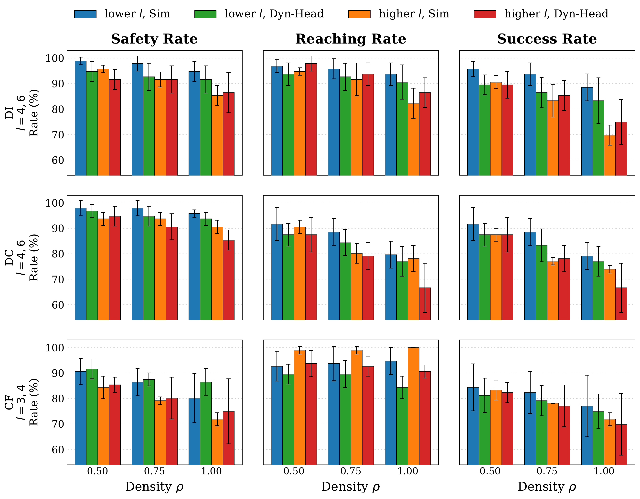
Zero-shot generalization across increased obstacle density $\rho$, defined as $N_\text{obs}/l^2$ for DI and DC and $N_\text{obs}/l^3$ for CF. The DI and DC models are trained with area size $l = 4$ and $N_\text{obs} = 8$, and the CF model with $l = 3$ and $N_\text{obs} = 6$; no retraining is performed. Both variants maintain competitive safety and success rates as the workspace scales, suggesting that the learned barrier critic generalizes to unseen obstacle configurations and larger environments.
Env. $\rho$ # Obs Safety Rate Reaching Rate Success Rate
Sim Dyn-Head Sim Dyn-Head Sim Dyn-Head
DI 0.508 98.96 ± 1.4794.79 ± 3.90 96.88 ± 2.5593.75 ± 4.42 95.83 ± 2.9589.58 ± 3.90
0.7512 97.92 ± 2.9592.71 ± 5.31 95.83 ± 3.9092.71 ± 5.31 93.75 ± 4.4286.46 ± 5.89
1.0016 94.79 ± 3.9091.67 ± 5.31 93.75 ± 4.4290.62 ± 6.75 88.54 ± 5.3183.33 ± 8.96
DC 0.508 97.92 ± 2.9596.88 ± 2.55 91.67 ± 6.4287.50 ± 4.42 91.67 ± 6.4287.50 ± 4.42
0.7512 97.92 ± 2.9594.79 ± 3.90 88.54 ± 5.3184.38 ± 5.10 88.54 ± 5.3183.33 ± 6.42
1.0016 95.83 ± 1.4793.75 ± 2.55 79.67 ± 5.3177.08 ± 5.89 79.17 ± 5.3177.08 ± 5.89
CF 0.5013 90.62 ± 5.1091.67 ± 3.90 92.71 ± 5.8989.58 ± 3.90 84.38 ± 9.2081.25 ± 6.75
0.7520 86.46 ± 5.3187.50 ± 2.55 93.75 ± 6.7589.58 ± 5.31 82.29 ± 8.2079.17 ± 5.89
1.0027 80.21 ± 9.6686.46 ± 5.31 94.79 ± 5.3184.38 ± 4.42 77.08 ± 12.0675.00 ± 6.75

Mean ± std over 32 environments and 3 seeds, 1024 timesteps.

Zero-shot generalization to larger and denser environments across two axes of out-of-distribution difficulty: obstacle density $\rho \in \{0.50, 0.75, 1.00\}$ and workspace size $l \in \{4, 6\}$ for DI and DC, and $l \in \{3, 4\}$ for CF. Rows are the dynamics (DI, DC, CF); columns are safety, reaching, and success rate. Each (seed, episode) instance is initialized at the highest density and lower-density variants are derived from the same instance by removing a random subset of obstacles, so that density is the sole varying factor.

Generalization in Action

Every clip below comes from a policy trained only on a $4 \times 4$ workspace with 8 obstacles. Nothing is retrained or fine-tuned. Moving left to right increases obstacle density $\rho = N_\text{obs}/l^2$; moving down enlarges the workspace, which lengthens the path to the goal and increases exposure to obstacles over the episode. Episodes run for 1024 control steps. The $8 \times 8$ rows go beyond the $l \in \{4, 6\}$ range reported in Table 2 and Fig. 2 above.

Double Integrator

$4 \times 4$ workspace — the training size

$\rho = 0.50$ · 8 obstacles

$\rho = 0.75$ · 12 obstacles

$\rho = 1.00$ · 16 obstacles

$6 \times 6$ workspace

$\rho = 0.50$ · 18 obstacles

$\rho = 0.75$ · 27 obstacles

$\rho = 1.00$ · 36 obstacles

$8 \times 8$ workspace — $4\times$ the training area

$\rho = 0.50$ · 32 obstacles

$\rho = 0.75$ · 48 obstacles

$\rho = 1.00$ · 64 obstacles

Dubins Car

$4 \times 4$ workspace — the training size

$\rho = 0.50$ · 8 obstacles

$\rho = 0.75$ · 12 obstacles

$\rho = 1.00$ · 16 obstacles

$6 \times 6$ workspace

$\rho = 0.50$ · 18 obstacles

$\rho = 0.75$ · 27 obstacles

$\rho = 1.00$ · 36 obstacles

$8 \times 8$ workspace — $4\times$ the training area

$\rho = 0.50$ · 32 obstacles

$\rho = 0.75$ · 48 obstacles

$\rho = 1.00$ · 64 obstacles

Ablations

Effect of the predictive horizon $H$ on Double Integrator, with history length fixed at $K = 12$. The $H = 1$ setting corresponds to pointwise barrier supervision without multi-step predictive lookahead, and gives the lowest safety rate. Increasing the horizon from $H = 1$ to $H = 6$ improves safety from $83.33\%$ to $95.83\%$, showing the benefit of enforcing barrier constraints over predicted rollouts rather than only at the next step. Increasing $H$ further does not consistently help at fixed history length, because longer rollouts accumulate dynamics-head prediction error and introduce more linearized barrier constraints in the SQP subproblem. We therefore use $H = 6$ with $K = 12$ in the main experiments.
Method $H$ Safety Rate Reaching Rate Success Rate
Ours (Dyn-Head) 183.33 ± 4.7890.63 ± 6.2578.12 ± 5.42
388.54 ± 5.8997.92 ± 1.4787.50 ± 6.75
695.83 ± 1.4789.58 ± 6.4288.54 ± 6.42
989.58 ± 5.3197.92 ± 1.4787.50 ± 6.75
1289.58 ± 3.90100.00 ± 0.0089.58 ± 3.90

Mean ± std over 32 environments and 3 seeds.

Freezing the transformer backbone and dynamics head after Phase 1. The frozen variant trains only the actor head and barrier critic in Phase 2, while Ours denotes the full training setup. The frozen dynamics head accumulates prediction error as the actor diverges from the pretraining distribution, and because attention is also frozen, the latent $z_t$ cannot adapt to the shifting action distribution — yielding inaccurate rollouts for barrier constraint evaluation. This motivates joint online training of all components.
Env. Safety Rate Reaching Rate Success Rate
FrozenOurs FrozenOurs FrozenOurs
DI 79.17 ± 8.2095.83 ± 1.47 96.88 ± 2.5589.58 ± 6.42 77.08 ± 9.6688.54 ± 6.42
DC 67.71 ± 2.2595.83 ± 2.95 100.00 ± 0.0092.71 ± 2.95 67.71 ± 2.2592.71 ± 2.95
CF 93.75 ± 5.1096.88 ± 2.55 89.58 ± 3.9092.71 ± 3.90 84.38 ± 9.2089.58 ± 6.42

Mean ± std over 32 environments and 3 seeds. Best mean values are bolded.

Robustness to dynamics perturbations on Double Integrator. All policies are trained on the unperturbed dynamics and evaluated without retraining, under a parametric velocity mismatch $\dot{p} = \alpha v$ and state-wise scaled process noise $\dot{x} = f(x,u) + w$, $w \sim \mathcal{N}(0, \Sigma_\sigma)$. Safety remains high across all tested $\alpha$; the lower reaching rate at $\alpha = 0.8$ is expected, since the robot moves more slowly and more often hits the episode time limit. Additive process noise is more challenging: safety stays above $92\%$ for moderate noise but degrades as the disturbance grows. The longer-history variant ($K = 32$, $H = 18$) tolerates larger noise better than the default. These are empirical robustness tests, not formal robust safety guarantees.
Perturbation Value $K = 12,\ H = 6$ $K = 32,\ H = 18$
SafeReachSuccess SafeReachSuccess
$\dot{p} = \alpha v$ 0.895.8475.0073.9694.7978.1375.00
0.996.8884.3784.3795.8386.4684.38
1.096.8889.5888.5497.9290.6389.58
1.195.8396.8893.7597.9294.7993.75
1.295.8396.8892.7194.7996.8892.71
$\dot{x} = f(x,u) + w$ $\sigma = 0$96.8889.5888.5497.9290.6389.58
$\sigma = 0.001$98.9689.5889.5895.8389.5888.54
$\sigma = 0.0025$92.7186.4683.3391.6788.5484.38
$\sigma = 0.005$73.9682.2968.7576.0484.3872.92
$\sigma = 0.0075$53.1279.1750.0063.5483.3361.46
$\sigma = 0.01$42.7178.1338.5446.8877.0843.75

Rates reported as percentages over 3 seeds and 32 environments.

BibTeX

@inproceedings{chauhan2026barrierformer,
  title     = {BarrierFormer: Transformer-Guided Predictive Barrier Enforcement for Safe Robot Control},
  author    = {Chauhan, Anandsingh and Garg, Kunal},
  booktitle = {Conference on Robot Learning (CoRL)},
  year      = {2026}
}